Question

How to number rows in excel spreadsheet

Answer 1

How to number rows in an Excel table: all methods The easiest way Reverse numbering "LINE" "PROGRESSION" Using formulas Conclusion Video

---

How to number rows in an Excel table: all methods

The Excel application provides ample opportunities for setting up and editing tables. Using the functionality of the program, you can also set the numbering of rows and columns. This can be useful when working with large databases. Let's figure out how to number rows in an Excel table in different ways.

The easiest way

For manual numbering, you do not need special program functions. And it’s difficult to call it completely manual, because you don’t have to enter each column number yourself. The user must do the following:

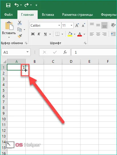
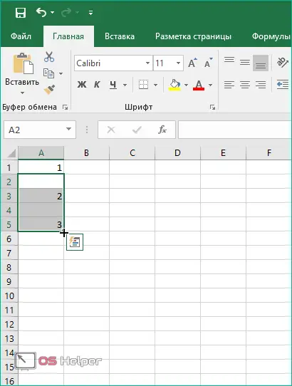
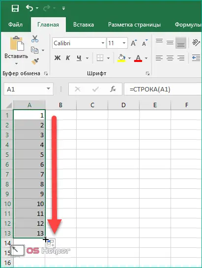
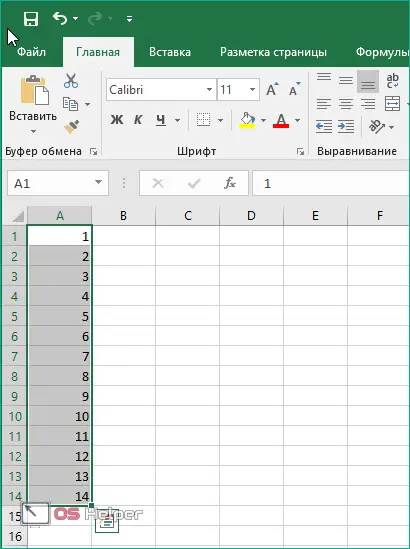
1. Enter a unit in the first cell. In the next cell - the number "2".

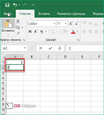
2. Select both cells and move the cursor to the lower right corner of the second cell so that it looks like a black cross.

3. Hold LMB and drag the cursor down to the required number of cells, then release the mouse.

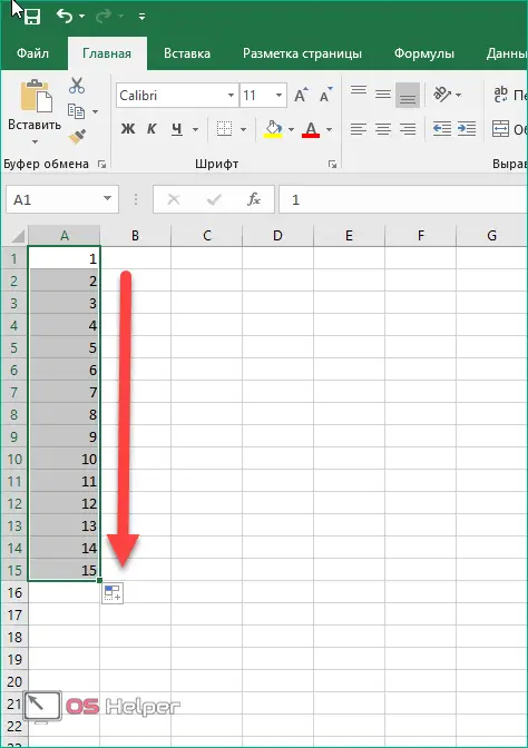
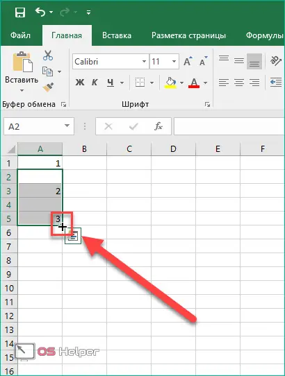
4. Now you will see the ordinal numbering of the column or row.

The second way to use this method:

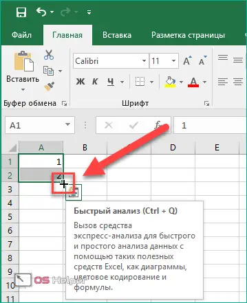
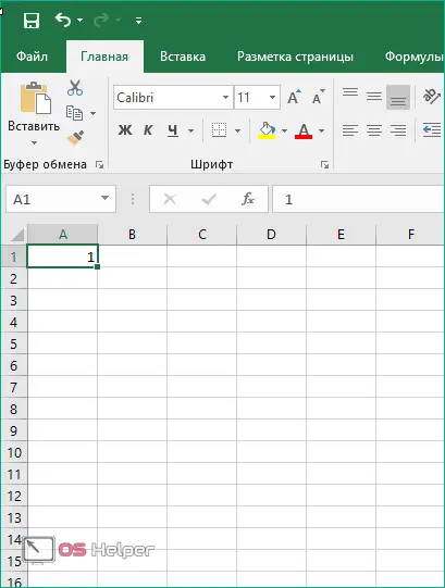
1. Again, enter "1" in the first cell.

2. Then put the cursor in the position of the black cross.

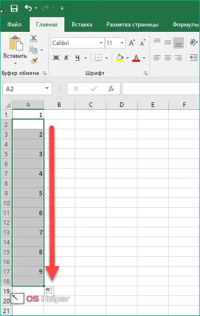
3. Hold the left [knopka]Ctrl[/knopka] on the keyboard together with LMB and drag the cursor down.

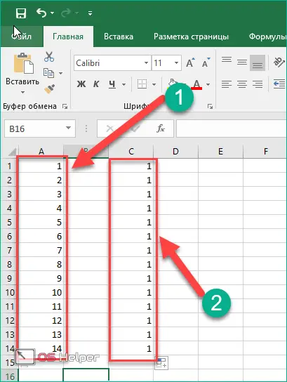
Attention! Release the [knopka]Ctrl[/knopka] key first, and then the left mouse button, and not vice versa (1). Otherwise, you will get a column of identical numbers (2):

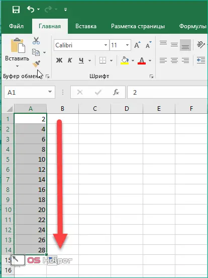
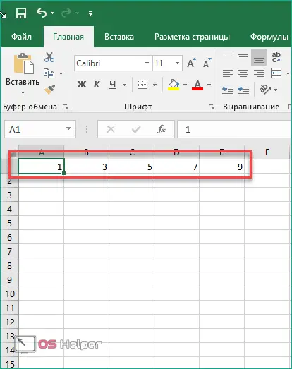
If you need a sequence with a certain step, for example, 2 4 6 8, then enter the first two digits of the series and follow all the steps from the previous instruction:

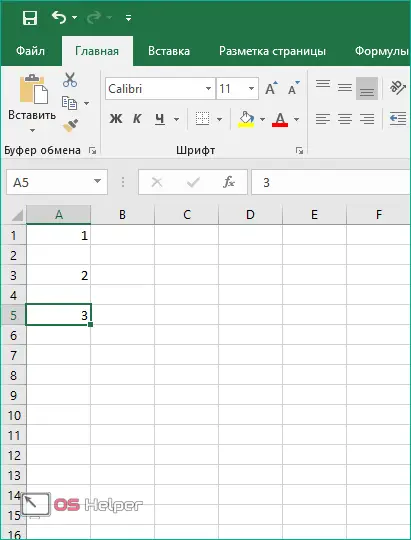
In order to make a table with a gap of one or more cells, you must:

1. Record the initial values ​​with the required interval.

2. Select all cells after the first value with the mouse.

3. Place the cursor in the lower right corner so that it takes the form of a cross.

4. Hold down the [knopka]Ctrl[/knopka] key and drag the cursor down. Now the table will be numbered as you intended.

Also Read:   How To Turn Off Compatibility Mode In Excel

Reverse numbering

To create a reverse order, you can use the above method:

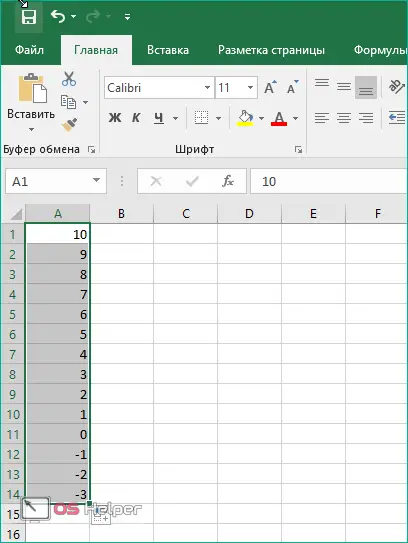
1. Enter the first numbers of the sequence, for example, 10 9 8.

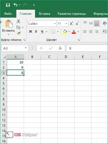
2. Select them and drag the handle down.

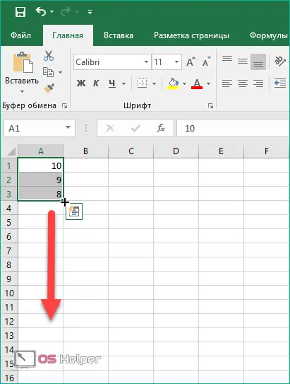
3. Numbers will appear on the screen in reverse. You can even use negative numbers.

"Excel" means not only a manual method, but also an automatic one. Manual dragging of the marker with the cursor is very difficult when working with large tables. Let's consider all the options in more detail.

"LINE"

Any operation in Excel is not complete without its counterpart in the form of a function. To use it, you must perform the following steps:

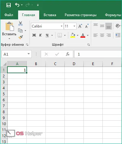
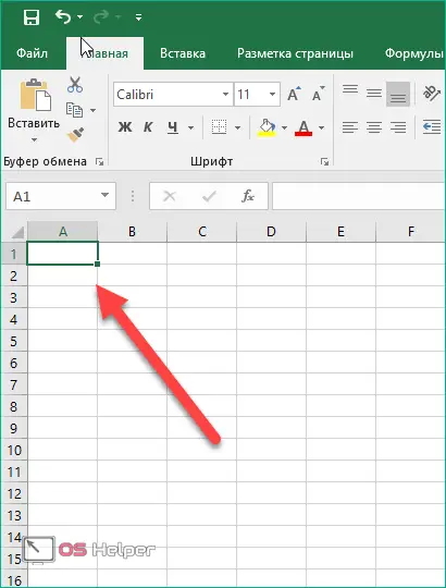
1. Select the starting cell.

2. In the function bar, enter the text "=ROW(A1)" and press [knopka]Enter[/knopka].

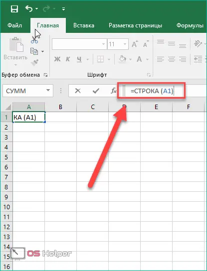
3. Now drag the edited cell with the marker down.

This option practically does not differ from the previous one in creating numbering in order. If you are dealing with a large amount of data and need a fast numbering method, then move on to the next option.

"PROGRESSION"

In this case, you do not have to manually drag the marker. The list will be created automatically according to the conditions you specified. Consider two options for using progression - fast and full.

In fast mode you need:

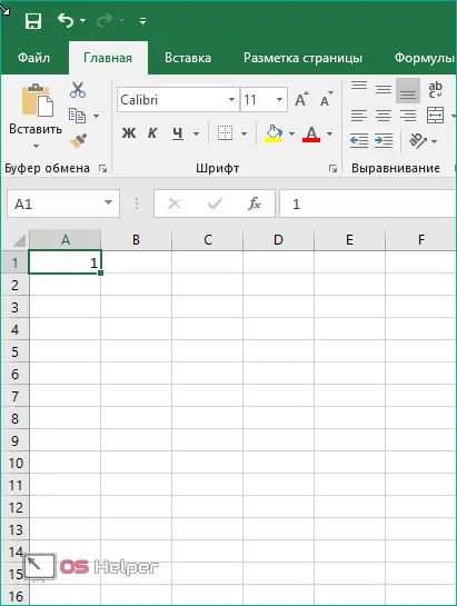
1. Enter the first digit of the future list.

2. Select the numbered cell and all subsequent ones that need to be numbered.

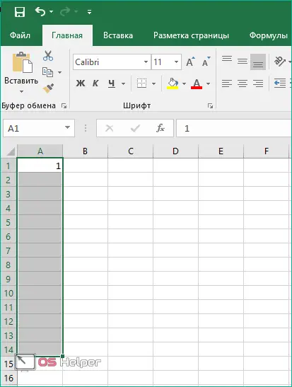
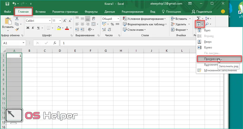
3. In the "Home" tab, click on the "Fill" button and select the "Progression" item in the menu.

4. In the window that opens, just click "OK".

5. Ready! The selected fields will turn into an ordered list.

If you need order with a certain step in the form of a gap between cells, then do the following:

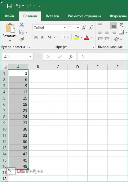
1. Enter the initial values ​​with the required step. For example, "3 6 9 12".

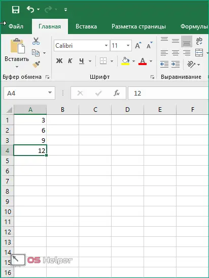
2. Highlight the filled cells that should be numbered.

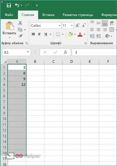
3. Open the "Progression" window again, as described in the previous instructions, and click "OK".

4. You will now see a numbered sequence in the document.

See also:   autofilter in excel

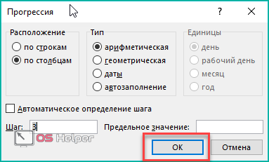
Now let's take a closer look at working with the "Progression" function:

1. First, enter the first number of the future list.

2. Go to the "Home" section, click on "Fill" and select "Progression".

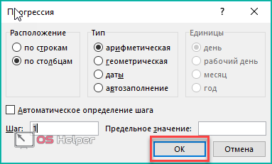
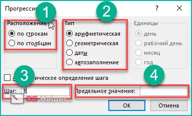
3. In the "Location" section, select the numbering direction (1), the type of progression (2), set the step for filling (3) and the limit value (4). Then click on "OK".

4. You will see a numbered table according to the given parameters. With this method, you do not have to manually drag the marker and enter the starting values.

Let's take a closer look at the types of progression by which you can create a numbered table:

• arithmetic sequence. This option implies ordinal numbers, for example, "10 11 12 13", etc.;
• geometric. With its help, a sequence is created by multiplying each previous value by a certain number. For example, a step equal to the number "3" will create the series "1 3 9 27", etc.;
• dates. A handy function for numbering rows and columns by day, month, and year.
• autocomplete. In this case, you manually specify a certain sequence, which the program continues by analogy.

Using formulas

And finally, the last way to fill. It is not very convenient, however, to fully describe the functionality of Excel, you need to talk about it. If you need a sequence with a certain step, then do the following:

1. Enter the starting number.

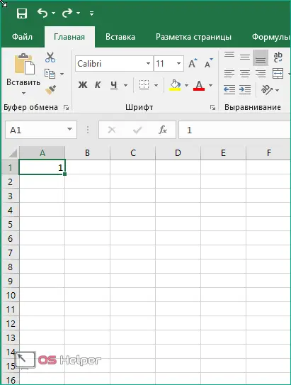
2. Activate the field where the list will continue with a certain step.

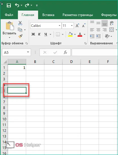
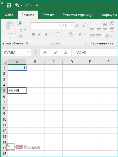
3. Here you need to set the formula. Put an "=" sign, then click on the first cell to make a link. Now specify the pitch, for example "+5" or "-2", etc. Press [knopka]Enter[/knopka] to finish.

4. Now select all cells from the first empty one to the entered formula. Using the marker in the lower right corner (without holding [knopka]Ctrl[/knopka]), drag the list down.

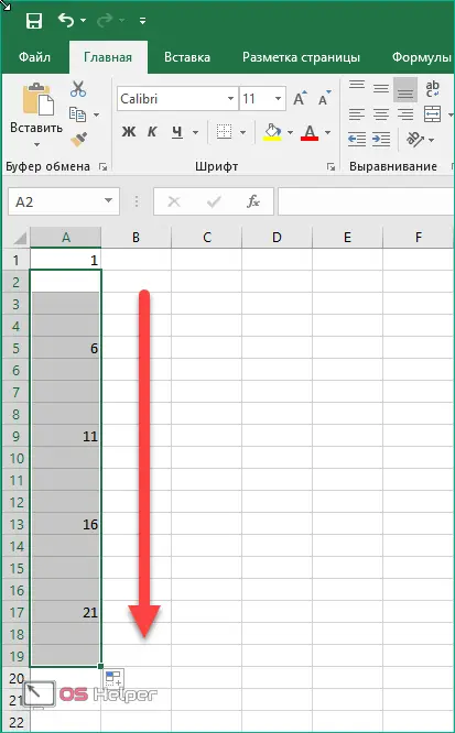
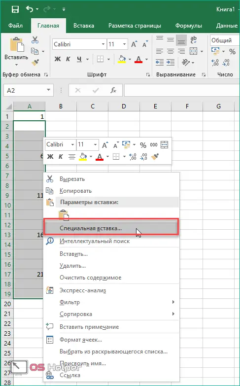
5. Next, you need to change the formulas obtained in the cells. To do this, select the entire list, copy and right-click. Select "Paste Special" from the menu.

Also Read:   Convert Excel to PDF

6. In the "Insert" section, select the "Values" item and click "OK".

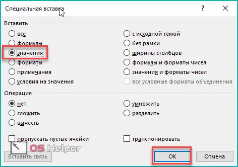
7. Now, instead of formulas, numbers will be written in the cells.

Conclusion

As you can see, creating numbered documents in Excel is possible in a variety of ways. Any user will find an option that will be convenient for him, whether it be functions, formulas, automatic or semi-manual method. In each case you will get the same result.

Video

In more detail and clearly on how to number tables in Excel, you can see in this video. It covers all the step-by-step actions from the presented instructions.