Question

How to Freeze a Row in Excel

Answer 1

How to freeze a row in Excel: step by step instructions Pinning the top cells Fixed header How to fix two rows Freezing a column How to fix two columns Locking Rows and Columns Simultaneously How to return everything as it was Pinning in Excel 2003 What to do if there is no "View" tab printout Conclusion Video instruction

---

How to freeze a row in Excel: step by step instructions

You can work with a huge amount of data in Microsoft Excel. On the one hand, it is very convenient. But on the other hand, in such situations there are certain difficulties. Since with a large amount of information, as a rule, the cells are very far from each other. And it does not contribute to readability. In such cases, the question arises: "How to freeze a row in Excel when scrolling?".

Pinning the top cells

It's very easy to make a hat permanent. To do this, you need to follow a few fairly simple steps.

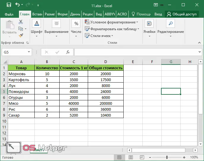
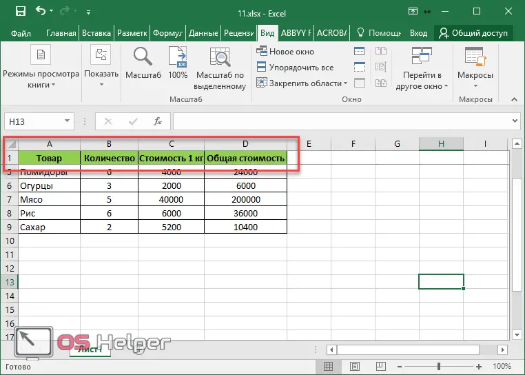
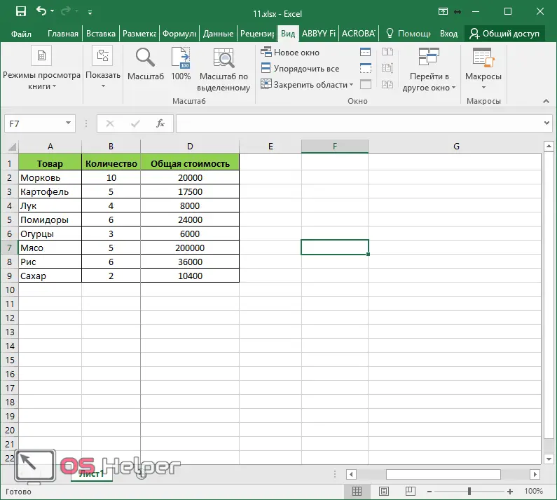
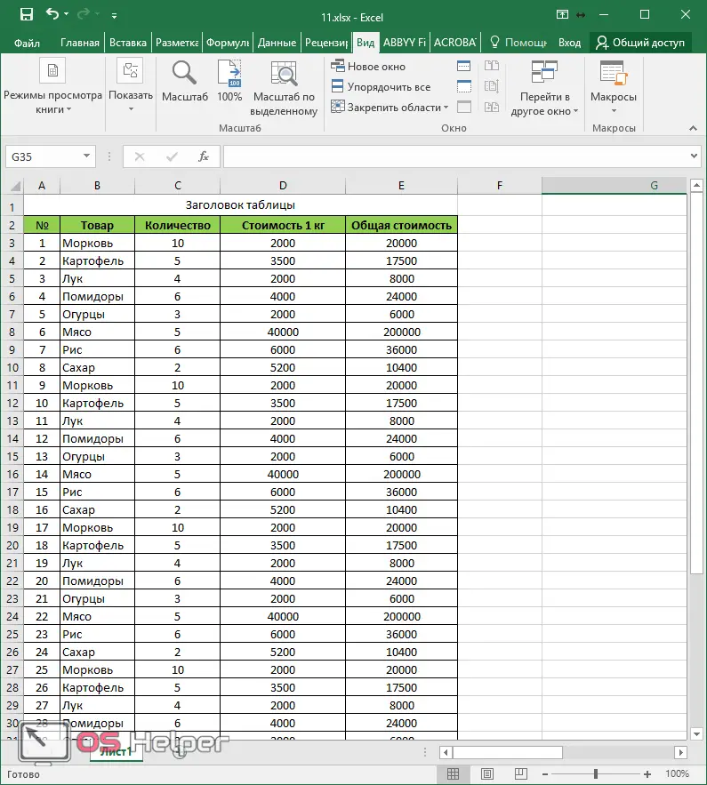
1. First, create a table with several rows and columns.

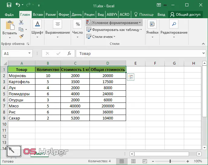
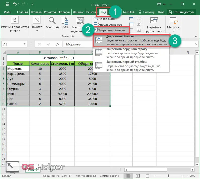
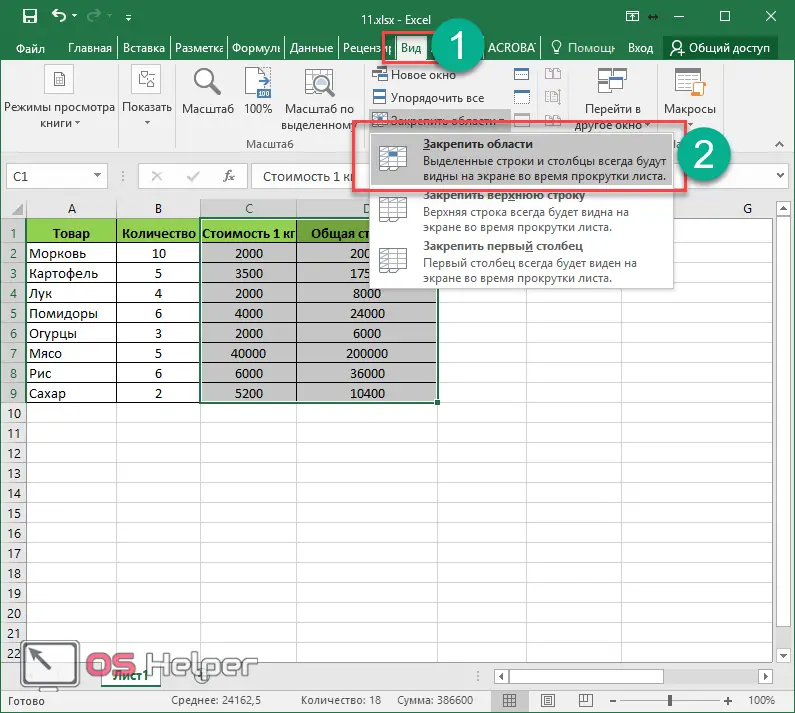
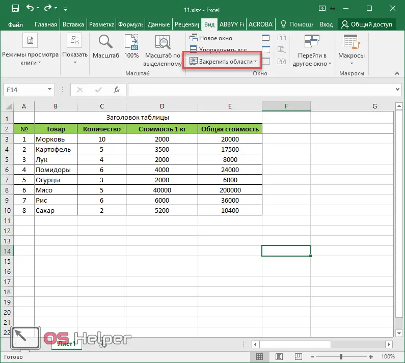
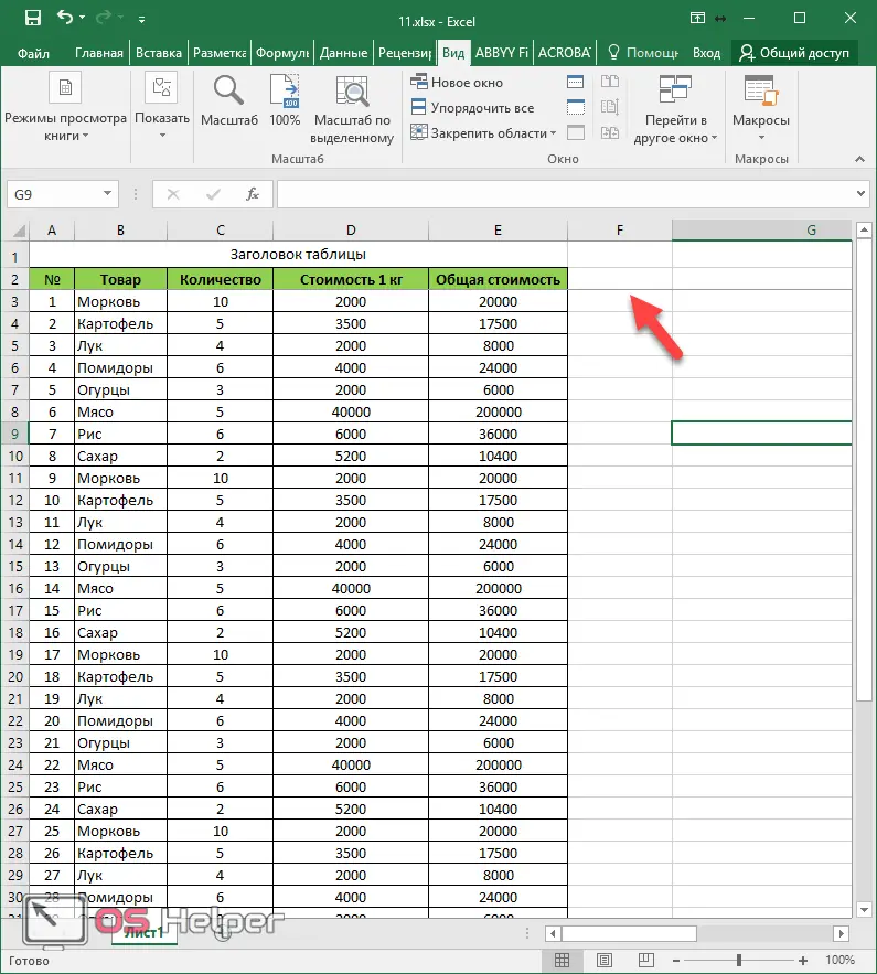
2. Now select the first line that you want to always see.

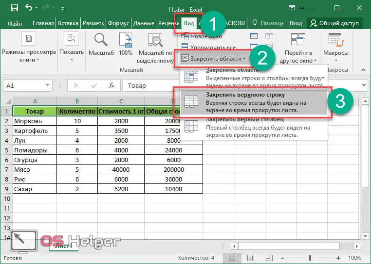
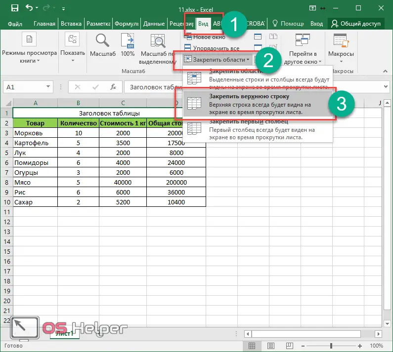
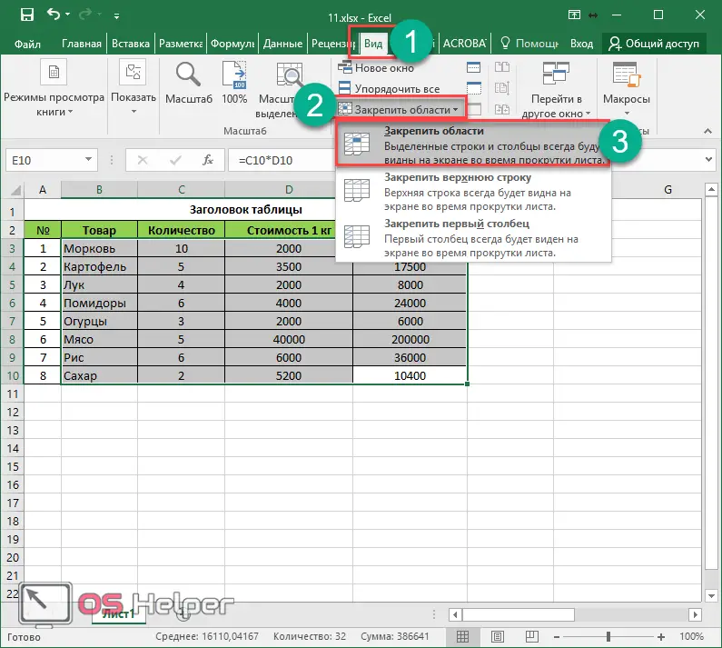
3. Click the "View" tab. Click the "Lock Areas" button. In the menu that appears, select the desired item.

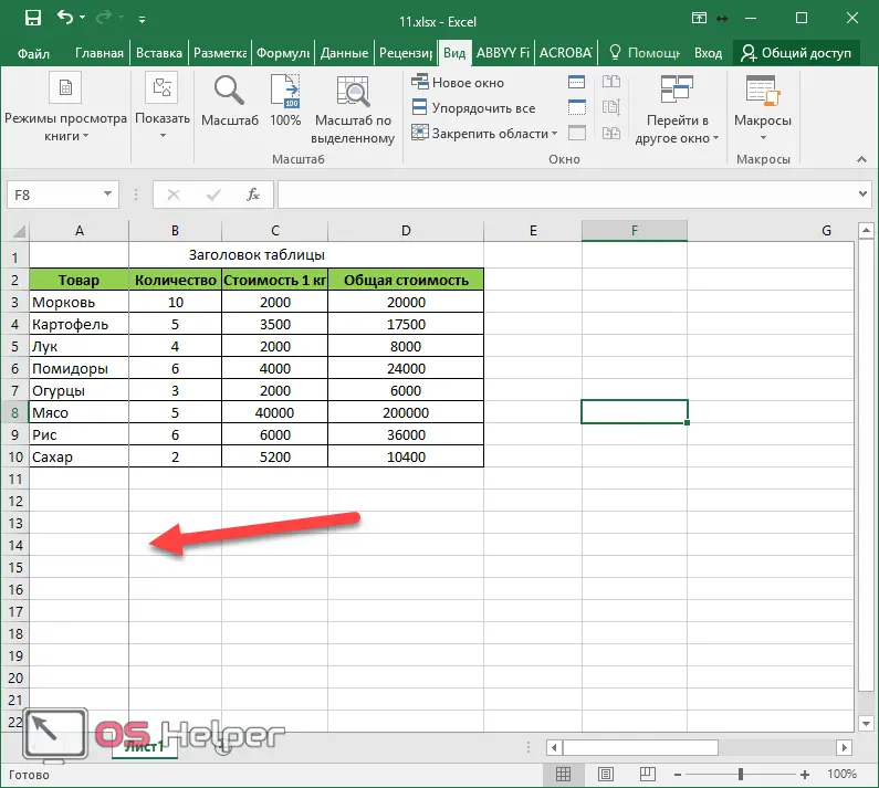
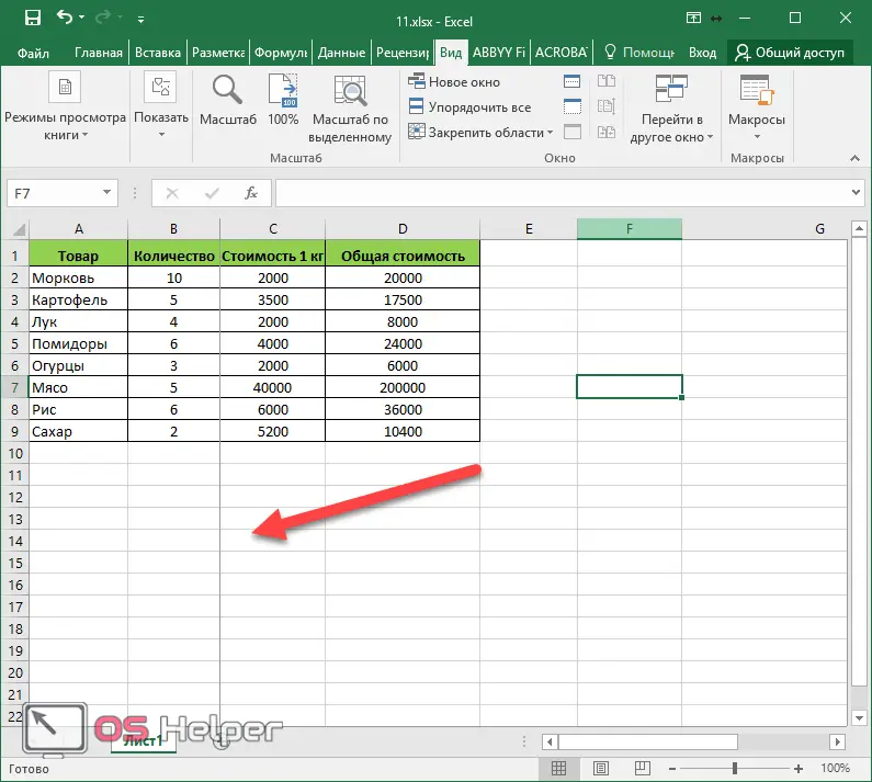
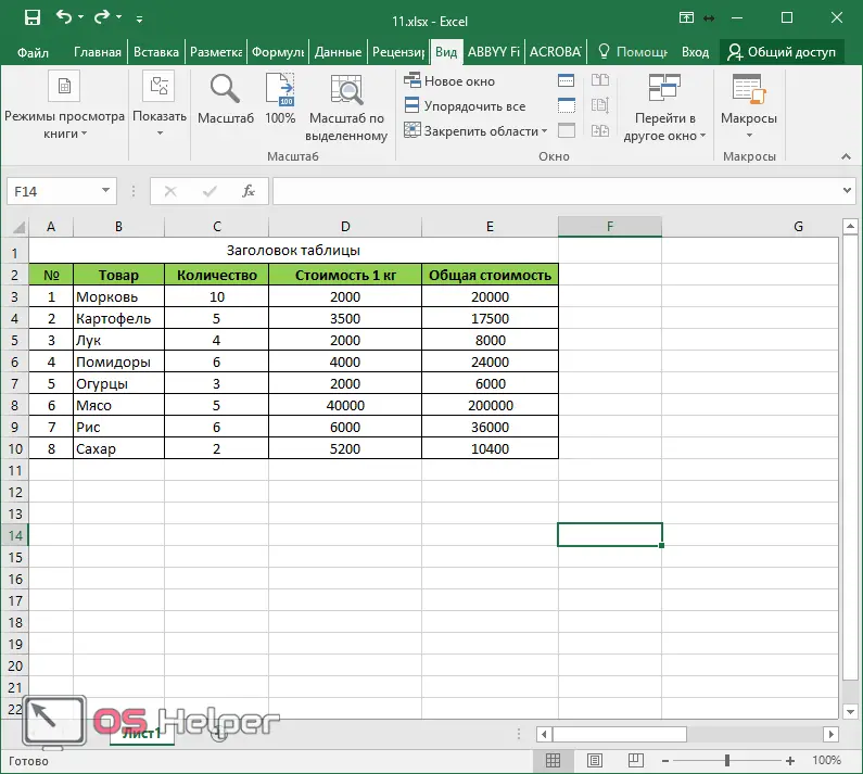
4. Immediately after that, a horizontal line will be displayed.

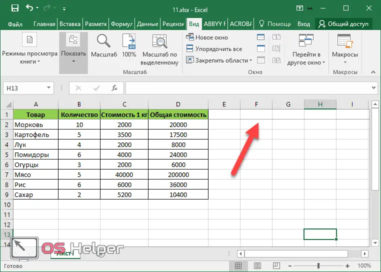
If it doesn't show up, then you did something wrong.

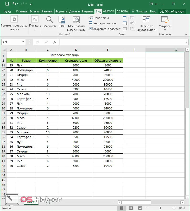
5. Now, after scrolling the sheet down, the desired row will remain in place.

Fixed header

This feature can be used for other purposes as well. For example, if you need to fix some text. This can be done in the following way.

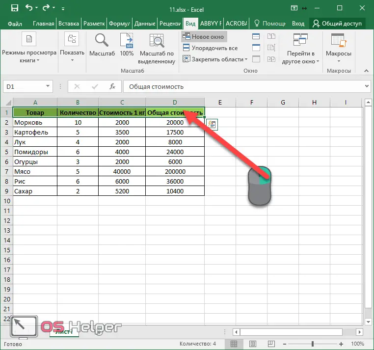
1. Let's use this table as an example. But we need to add a title. To do this, select the first line and right-click the mouse.

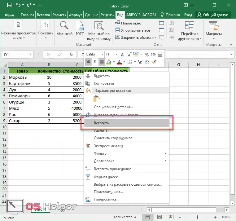
2. In the context menu that appears, click on the "Insert ..." item.

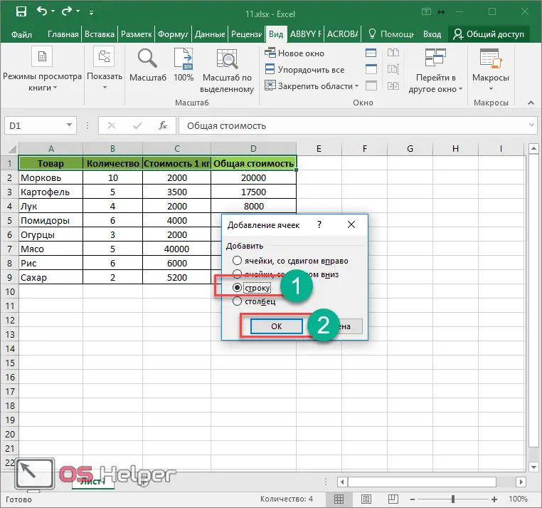
3. Next, select the third item and click on the "OK" button.

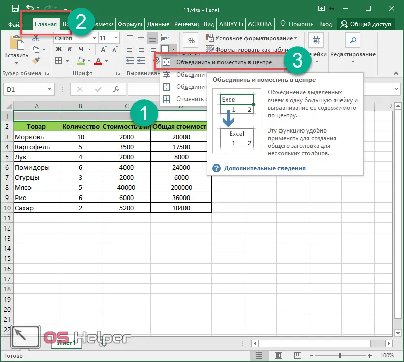
4. Highlight the line that appears. Go to the "Home" tab. Click on the "Merge and Center" button.

See also:   How to make numbering in order automatically in Excel

5. Write something there.

6. Again, go to the "View" tab and fix the top row.

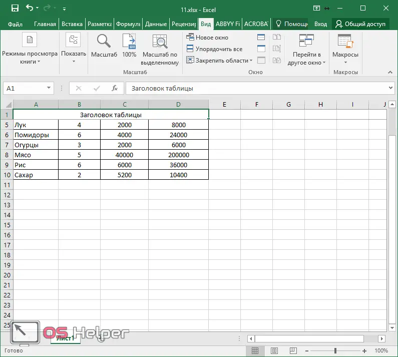
7. Now your title will always be at the top, even when scrolling down the page.

How to fix two rows

But what if you need to make the header and title fixed? It's pretty simple.

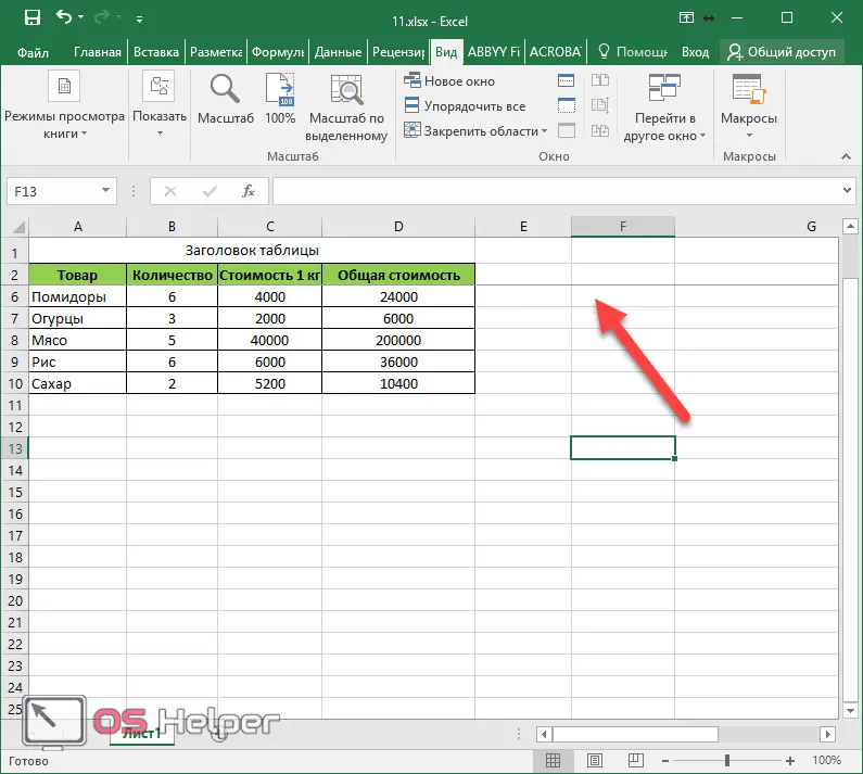
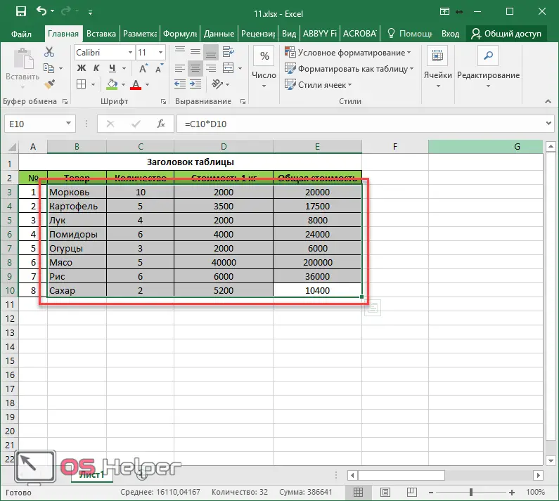
1. Select the remaining cells, except for the top two.

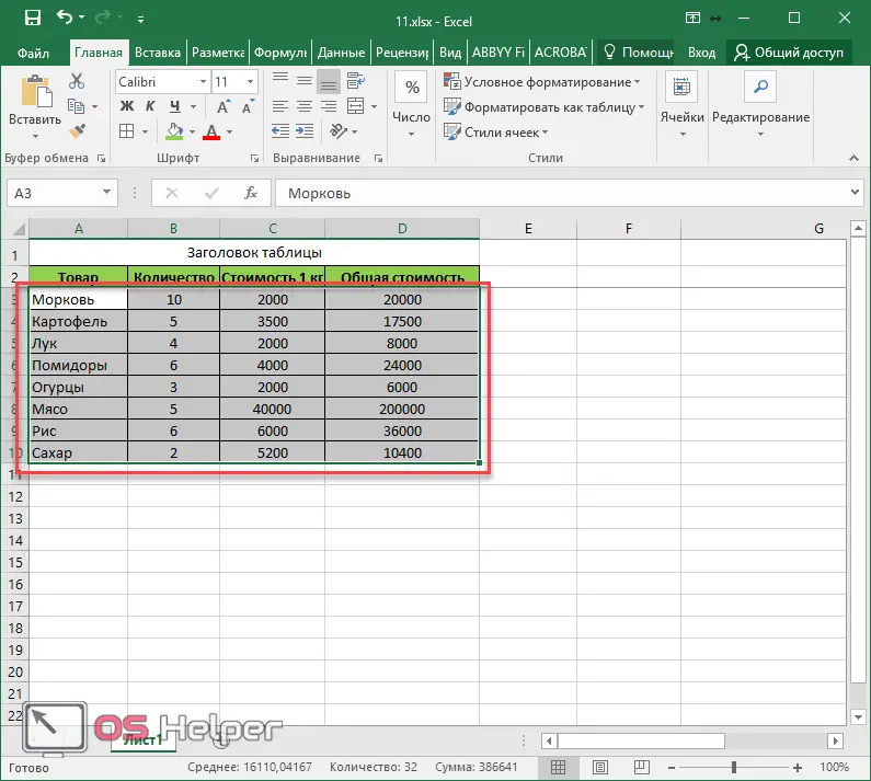
2. This time we click on the first item, and not “pin the top line”.

3. After that, the line after the second line will be highlighted. Now when you move the page down, everything above will be fixed.

Freezing a column

Columns are also easy to fix. To do this, you must perform the following steps.

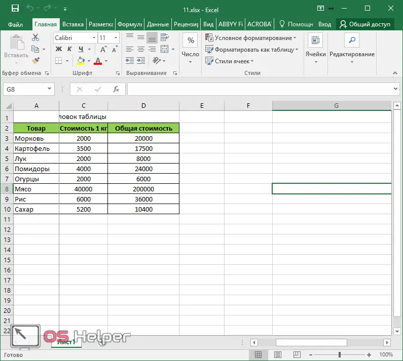
1. Select the left side cells.

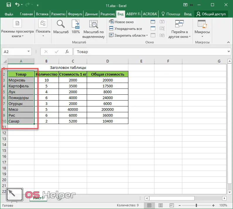
2. Open the "View" tab. Expand the menu for fixing. Then select the desired item.

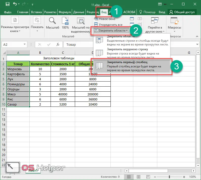
3. After that, you will have a vertical line that will limit the fixed area.

4. Now when scrolling the page to the right, the first column will remain in place.

How to fix two columns

If you need to increase the number of fixed cells, you need to do the following.

1. Select the remaining cells.

2. Open the View tab and select Freeze Panes.

3. Now the fixed vertical line will be after the second column.

4. And everything to the left of it will be motionless.

Locking Rows and Columns Simultaneously

In order to fix horizontal and vertical cells, you need to do the same as described above. You just need to use both methods at once.

1. First, select a workspace that should always move.

2. Click the "View" tab. Expand the menu already familiar to us and select the first option.

3. After that, you will have two lines: horizontal and vertical.

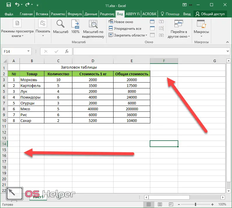
Now everything that is above and to the left of them will stand still.

How to return everything as it was

In order to undo all the actions described above, you need to do the following.

1. Click the "Freeze Areas" button again.

See also:   Create a table in Excel: instructions for dummies

2. This time, the option "Unpin areas" will appear in the menu options.

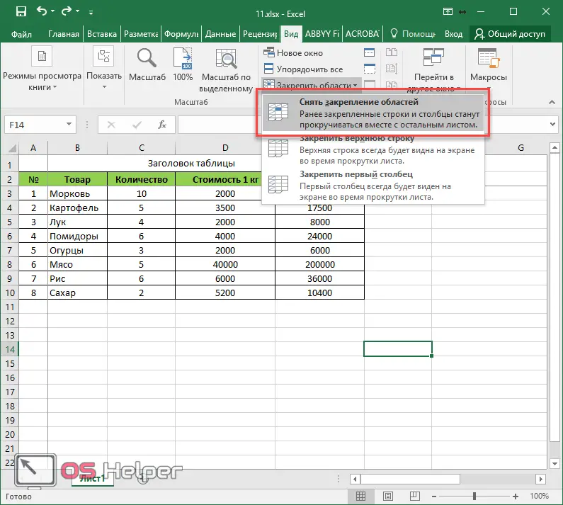
3. By clicking on this item, all bounding lines will disappear.

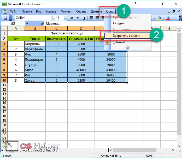
Pinning in Excel 2003

Everything that was described above is suitable for the new versions of 2007, 2010, 2013 and 2022. In old Excel, the menu is located differently. You can pin an area in the "Window" menu section.

Everything else works on the same principle as it was said earlier.

What to do if there is no "View" tab

Some users do not have this item in the menu. How to be? Help comes online help from Microsoft. According to her, the Excel Starter version does not have the ability to freeze panes.

The rest of the features and limitations in the "Starter" can be found here.

printout

In order to demonstrate what happens when the pages are printed, let's do the following steps.

1. First, let's increase the number of cells in the table.

2. Fix the header and title.

3. Scroll down and make sure they are stationary and have hidden cells underneath them.

4. Now press the hotkeys [knopka]Ctrl[/knopka]+[knopka]P[/knopka]. In the window that appears, you need to make sure that the printer is ready for use. After that, click on the "Print" button.

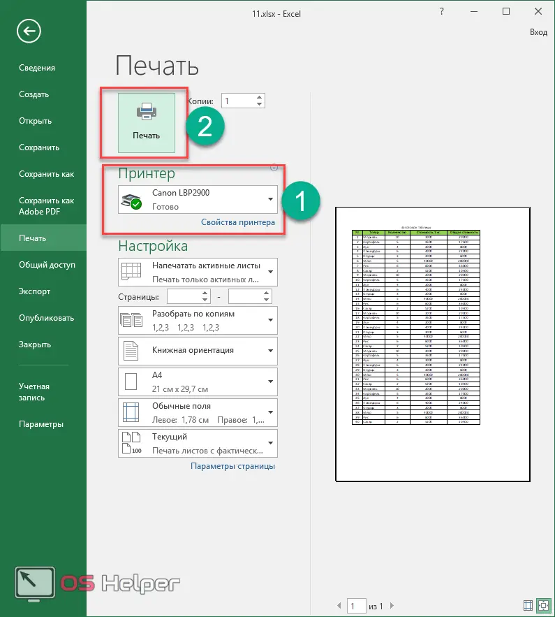
5. See the result of what the printer printed.

As you can see, everything is in its place.

Conclusion

This article showed you how to fix the desired rows and columns so that they remain stationary when working with a large amount of information. If something didn’t work out for you, then most likely you select the wrong area. You may need to experiment a bit to get the desired effect.

Video instruction

For those who still didn’t succeed, a short video with additional comments is attached below.