Question

How to merge cells in Excel

Answer 1

How to merge cells in Excel: easy ways Toolbar Cell Format Duplicate Fragments Format by paragraph Merge without data loss How to undo a merge What to do if the button is disabled Conclusion Video instruction Extended capabilities Toolbar Context menu

---

How to merge cells in Excel: easy ways

Excel is a very powerful spreadsheet tool. That is why it is so in demand among people of various professions. At the same time, not everyone knows how to combine cells in Excel. Actually, it's easy. There are a large number of ways. Let's consider them in more detail.

Toolbar

In order to connect several cells in the simplest way, you must do the following.

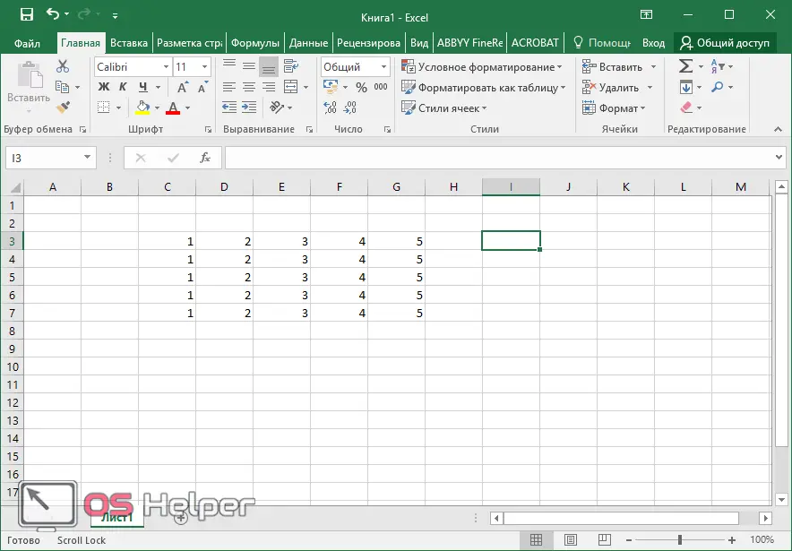
1. Put any values ​​in several cells.

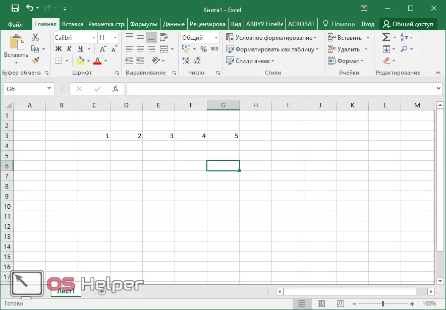
2. Now select this entire line.

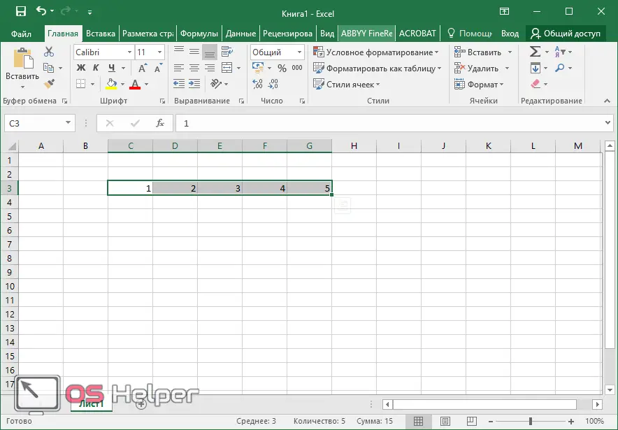
3. Then click on the "Merge and Center" icon.

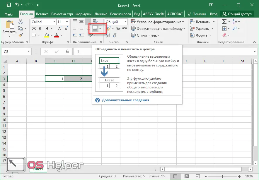
4. After that, you will see the following.

You are warned that all information, except for the one in the first cell, will be lost.

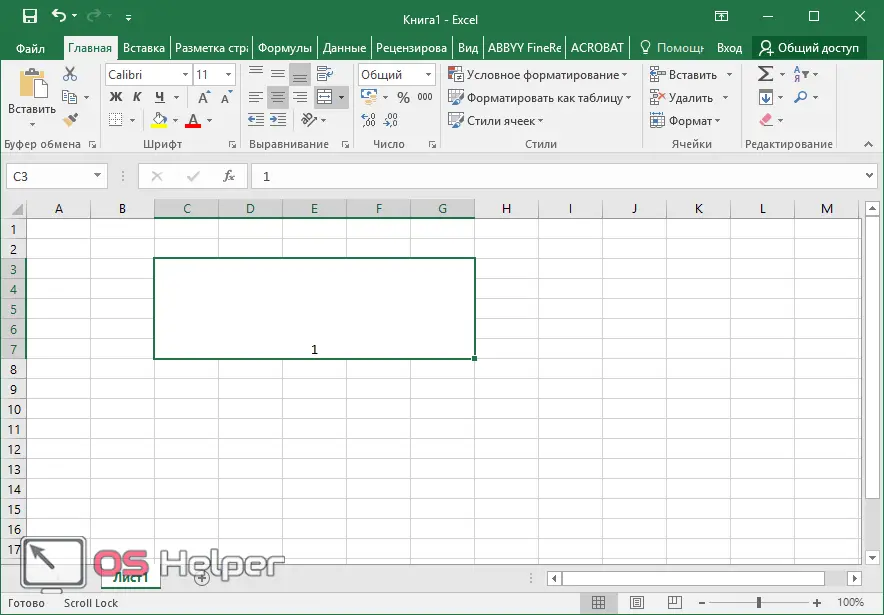
5. You must agree to this condition. To do this, click on the "OK" button. The result of the actions described above will be a long string, in which only the number 1 remains, since it was in the first selected fragment. In addition, the content is aligned to the center.

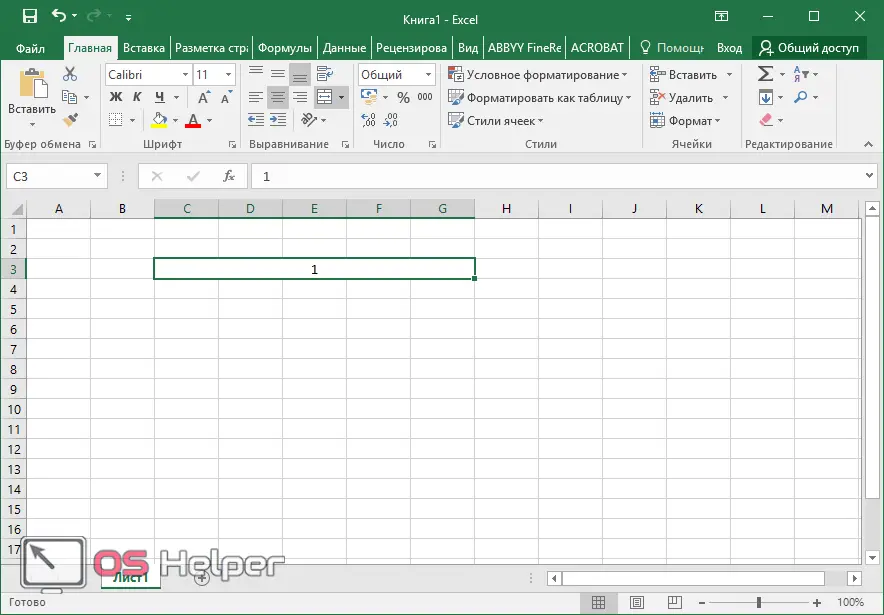
It should be noted that all other information will be destroyed. Therefore, usually only empty cells are merged.

Extended capabilities

In order to demonstrate what can be done using the toolbar, our table will need to be significantly enlarged.

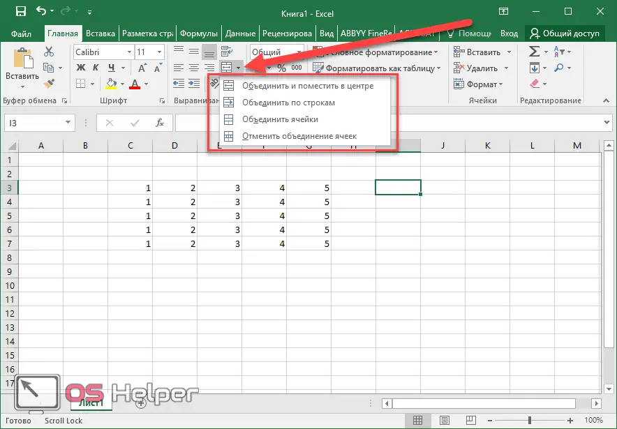
If you click not on the button, but on the “triangle” next to it, you can see additional menu items.

Merge and center

Select all items and click on the corresponding menu item.

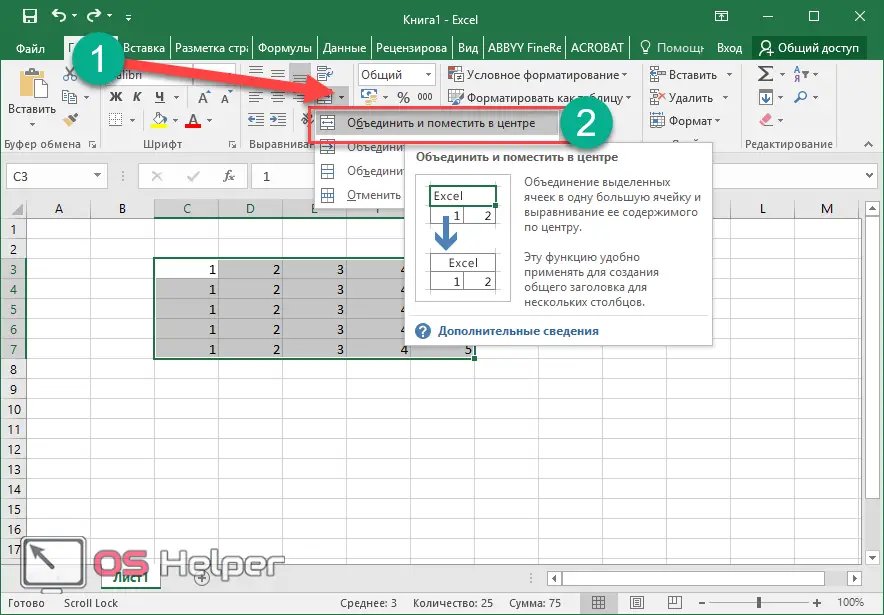
You will again be warned about the loss of values. We agree with this.

As a result, you will get the following result.

Merge by lines

Select the entire table and click on the second item.

See also:   The set of values ​​​​that can be entered in an Excel cell is limited: a solution to the problem

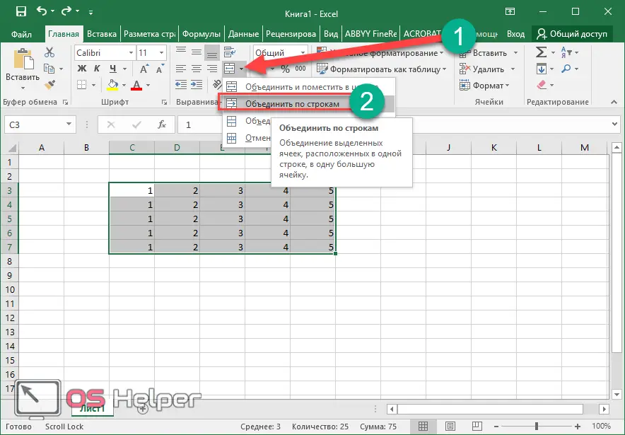
After that, you will see the standard warning. But note that the number of popups will match the number of rows in your table.

As a result of this, you will get many rows consisting of several merged cells.

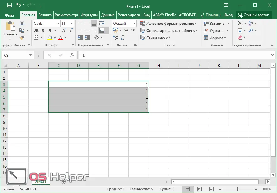
In our case, duplicate data is due to the fact that all rows were the same.

Merge Cells

To demonstrate this capability, the following steps need to be taken.

1. Select a few items, not the entire table.
2. Click on the triangle icon to bring up an additional menu.
3. Select the appropriate item.

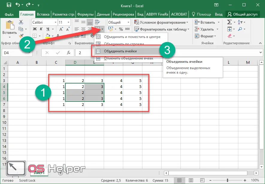
4. We agree that as a result of the operation, only the contents of the upper left cell from the entire selected range will be saved.

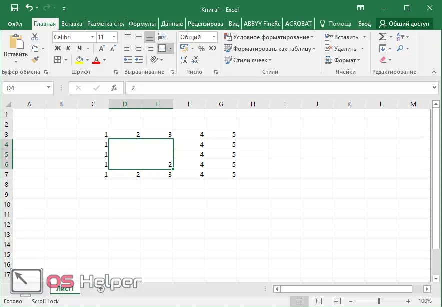
5. As a result, we get a large rectangle with only one number.

Cell Format

The steps described above can also be repeated using the context menu.

1. Select several cells with text or any other content.
2. Do the right mouse click on the active elements.
3. Then select "Format Cells".

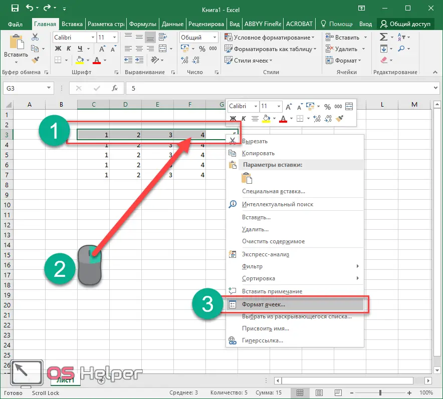
4. As a result, the following window will appear.

5. We are interested in two sections here:
   • alignment (here you can specify any suitable option);

• display (here be sure to check the box next to "Merge cells").

6. At the end, click on the "OK" button.

7. We agree with the warning.

Thanks to this, we get the following result.

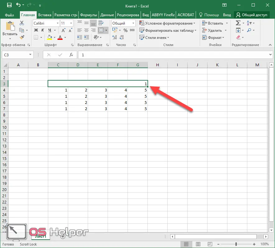
Using this mechanism, you can combine any number of elements both vertically and horizontally. The main thing is to select the desired range before calling the context menu.

Duplicate Fragments

If you already have rows that consist of several cells, you can always easily copy them. In this case, all formatting will be completely the same. To do this, let's do a few simple steps.

1. Select the existing merged fragment.

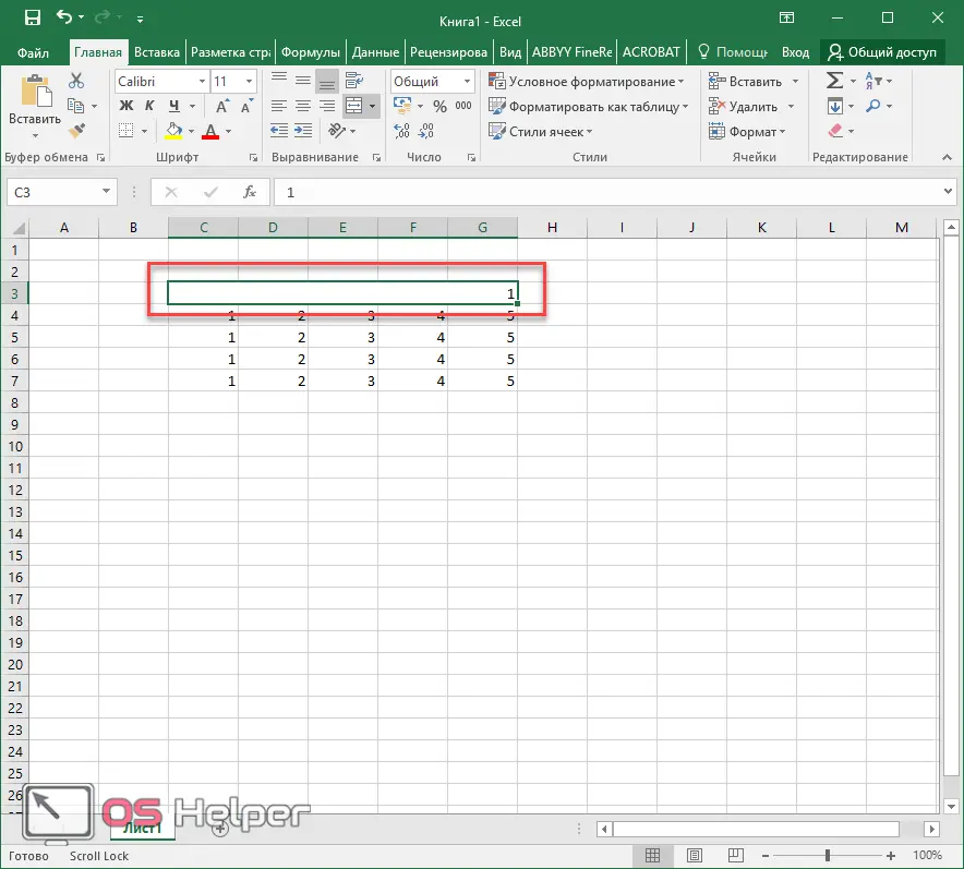
2. Press the hotkeys [knopka]Ctrl[/knopka]+[knopka]C[/knopka] (a dotted frame should appear).

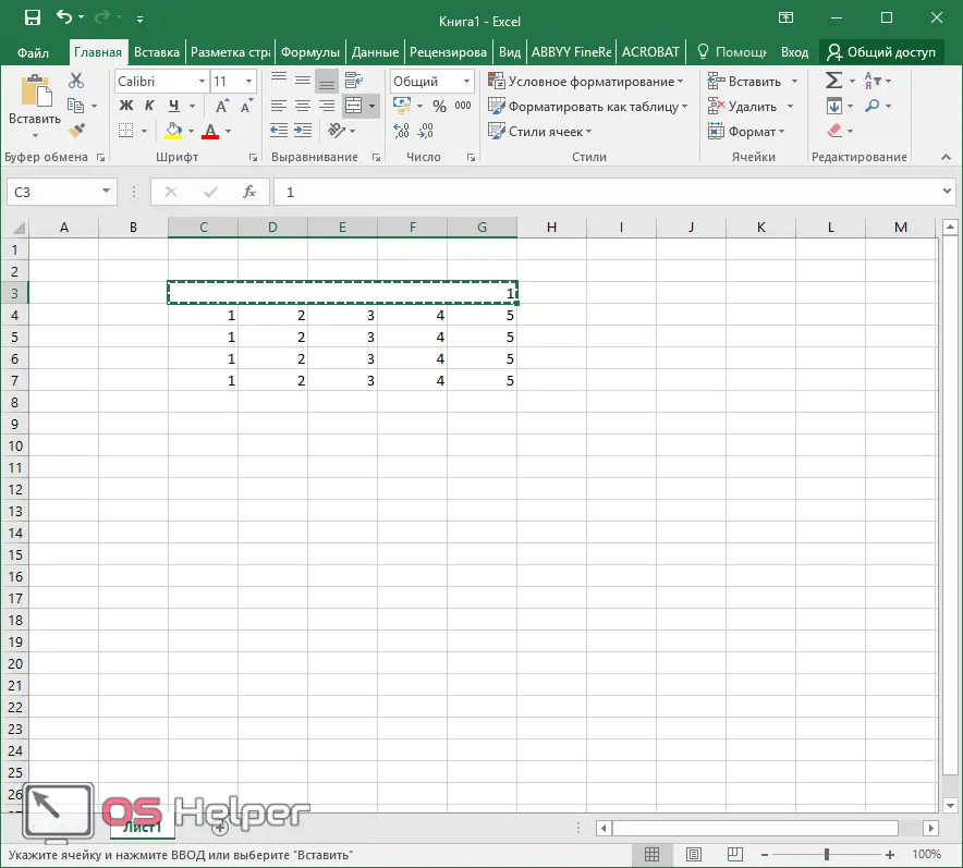
3. Click on some other element.

See also:   How to fix the table header in Excel

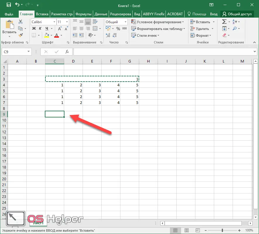
4. Press the hotkeys [knopka]Ctrl[/knopka]+[knopka]V[/knopka].
5. As a result, we get an exact copy of the original string.

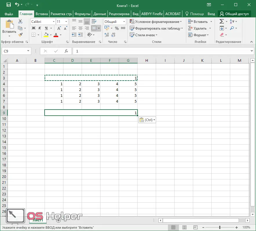
Thanks to this method, you can copy any number of "modified" cells.

Format by paragraph

You can copy the design in another way. This is made even easier.

1. Select the line whose appearance needs to be duplicated.
2. Click on the brush icon. Immediately after that, the cursor should change its appearance.

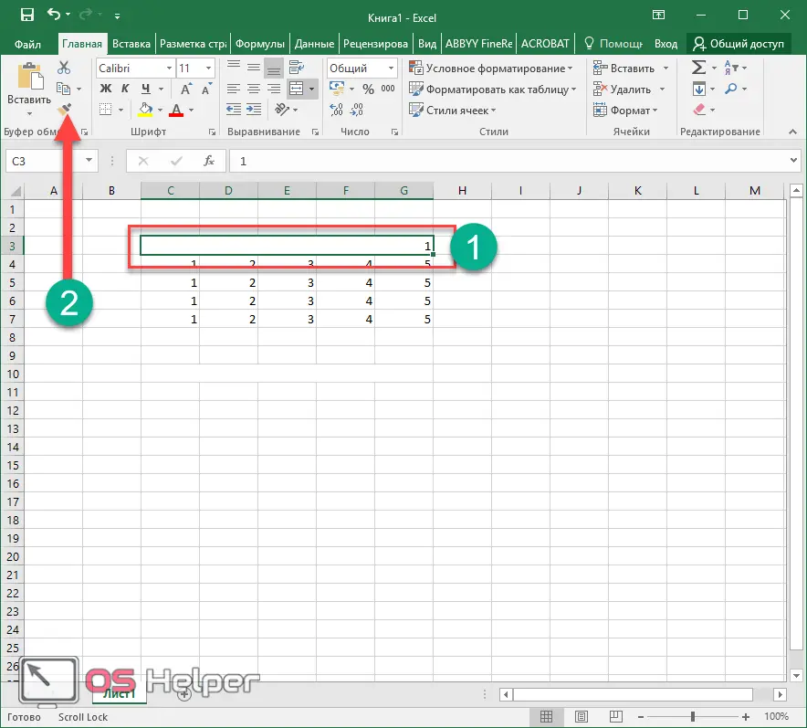
3. Then click on the element you want to transform.

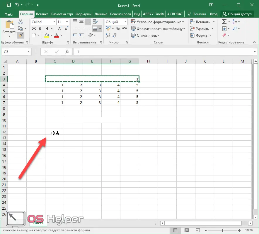
4. As a result of this, all cells that are to the right of the selected one will be merged. The number of combined cells coincides with the original source.

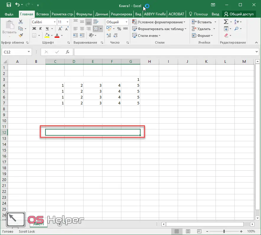
Merge without data loss

In the methods described above, information was deleted in all other elements of the table, except for the first one. You can use the built-in functions of Microsoft Excel to create a string from several fragments and at the same time preserve the original data.

1. Move the cursor to the desired location. Click on the "fx" button.

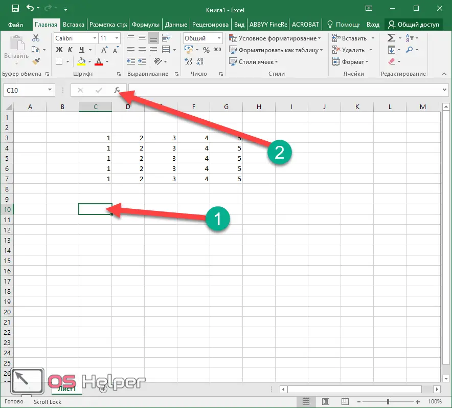
2. Immediately after that, you will see a window for inserting a function.

3. You need to change the category to "Text".

4. Next, find the "Link" function in the list. Select it and click on the "OK" button.

5. Immediately after that, a new window will appear in which you need to specify the function arguments. Links to elements can be entered manually.

6. But the easiest way is to just click on them one by one. First, click on the "Text 1" field.

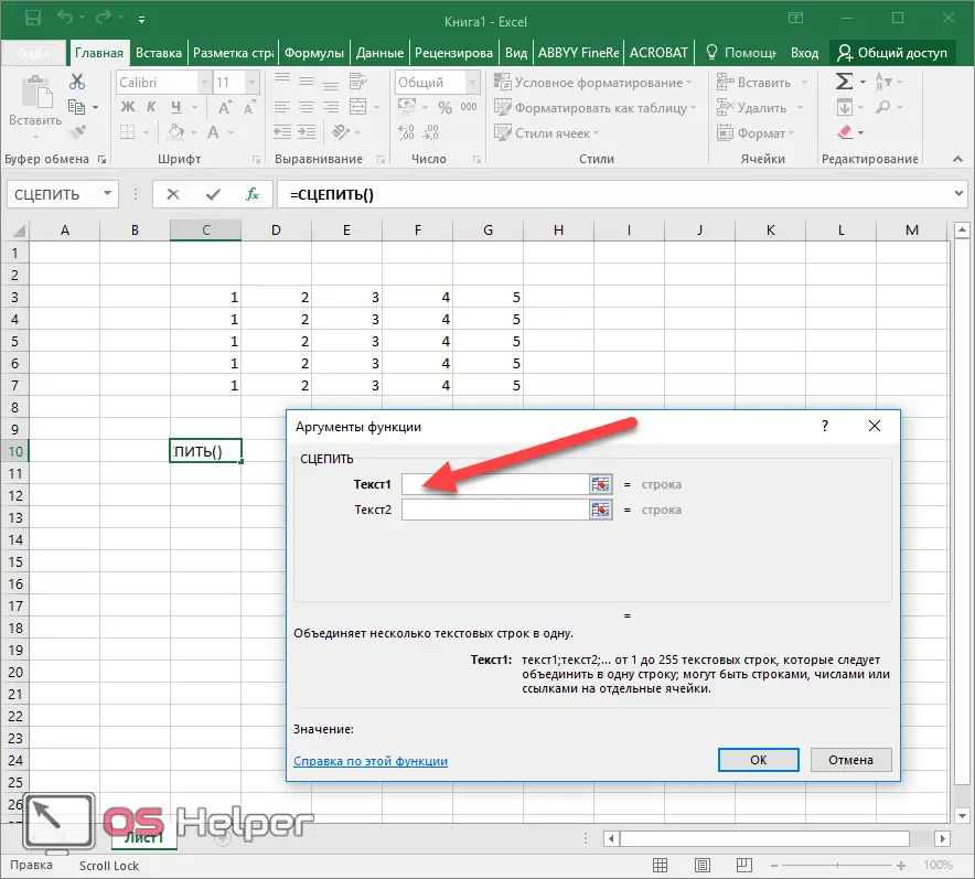
7. Then to the first element of the desired line (the data will be substituted automatically).

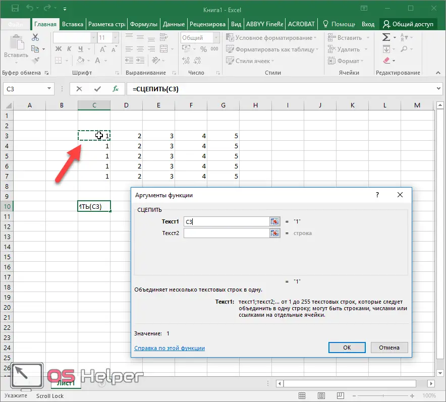
8. Then go to the "Text2" field.

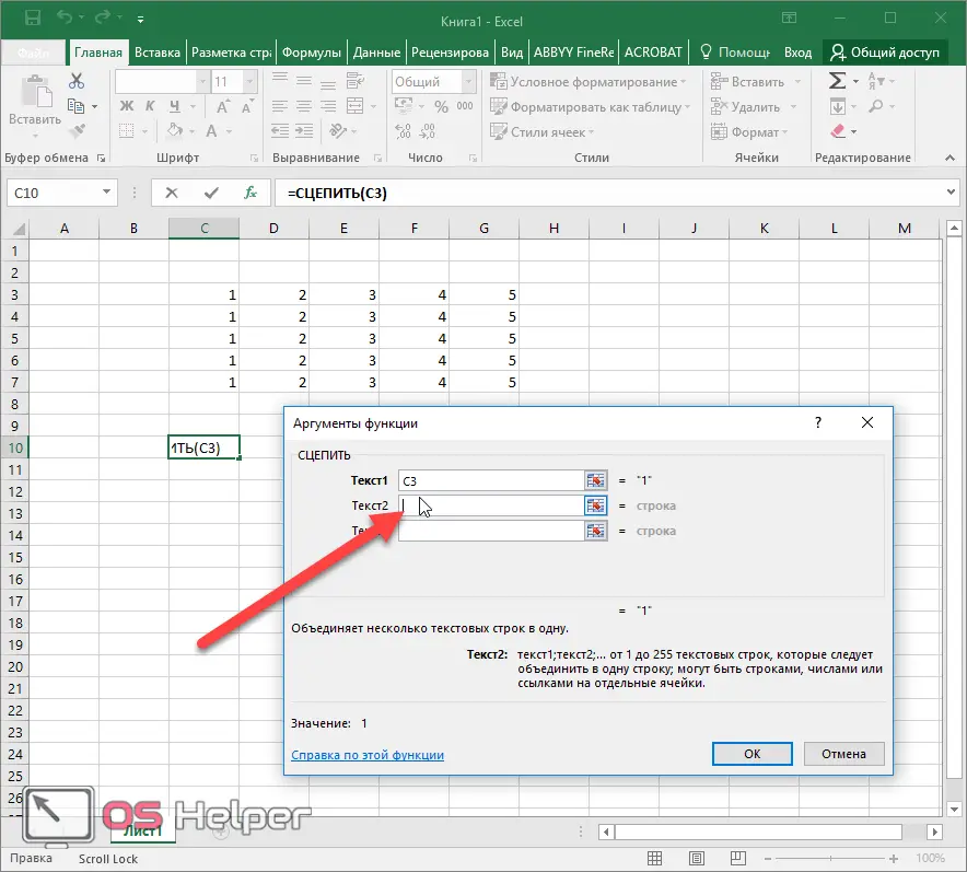
9. This time, click on the next cell.

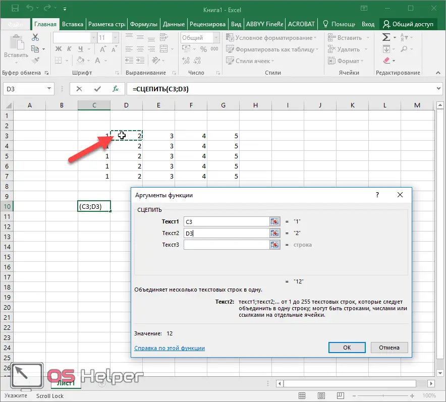
Each time you add a new link, additional input fields will appear. Thus, you need to drive in the values ​​\u200b\u200bto the very end of the line.

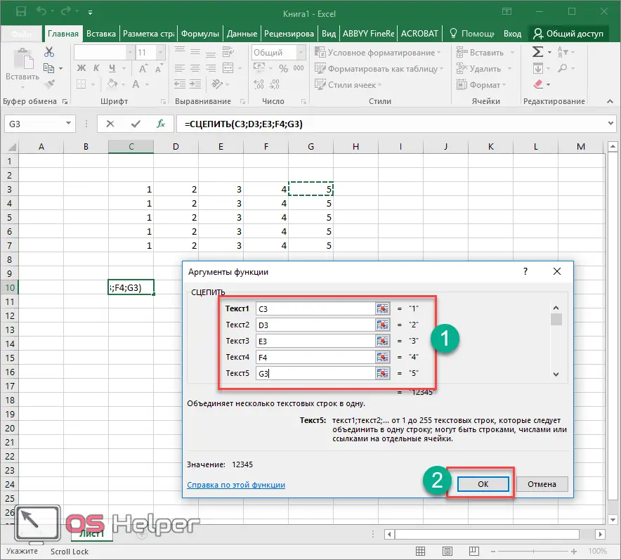
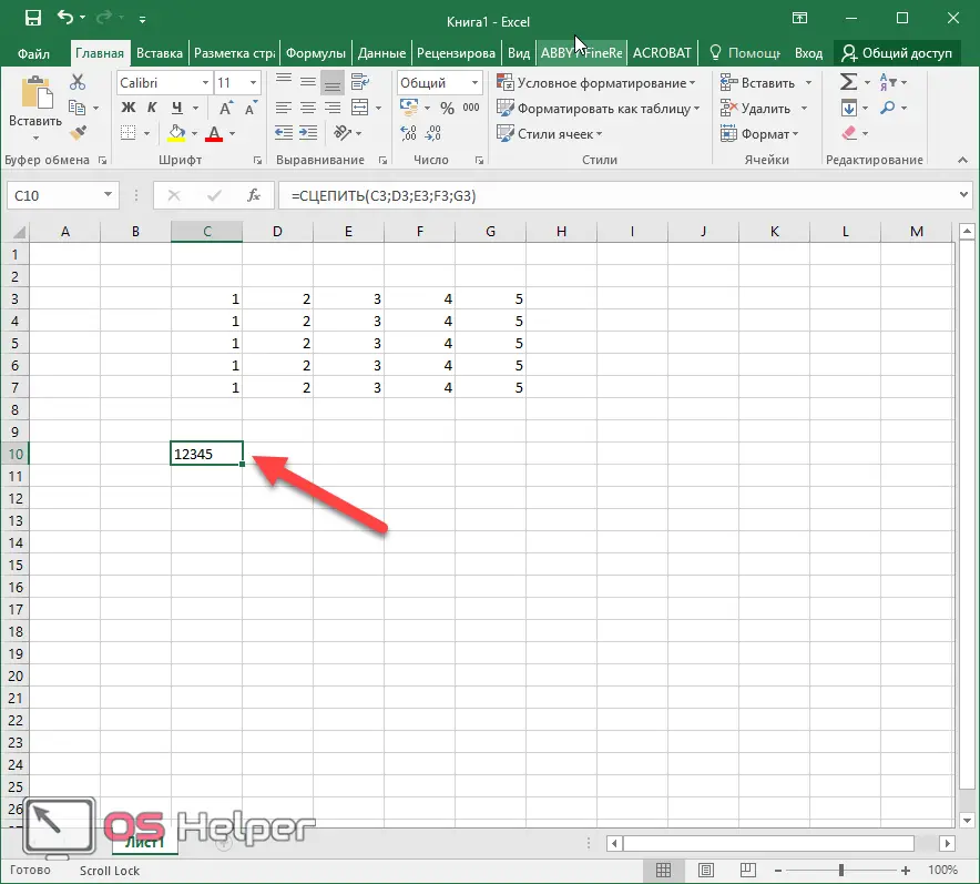
When you're done, just click on the "OK" button. As a result of this, you will get a string containing the values ​​of all the above fragments.

How to undo a merge

If you have joined more than you need, or the wrong line at all, then reverting everything back is very simple:

• for this, just press the hot keys [knopka]Ctrl[/knopka]+[knopka]Z[/knopka];
• or click on the icon to undo the last action on the quick access toolbar.

See also:   How to add a row in Excel

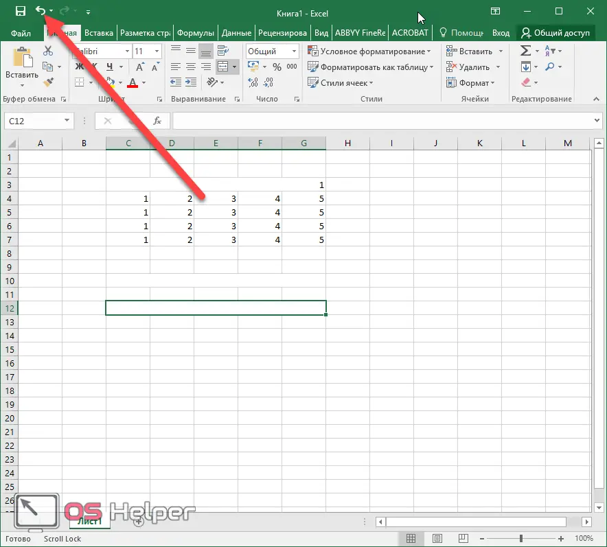
But there are other cases when you need to split a string that was merged a long time ago. Or you have a large number of them and they were created at different stages of working with text in the table. In this case, undoing the last action will not help.

For such cases, there are two other methods. Let's consider them in more detail.

Toolbar

Return everything as it was possible in the same place where the union takes place.

1. Select the required part of the table. On the Home tab, click on the triangle icon. Choose the last item.

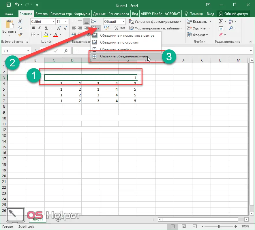
2. Thanks to this, everything will return to its original state.

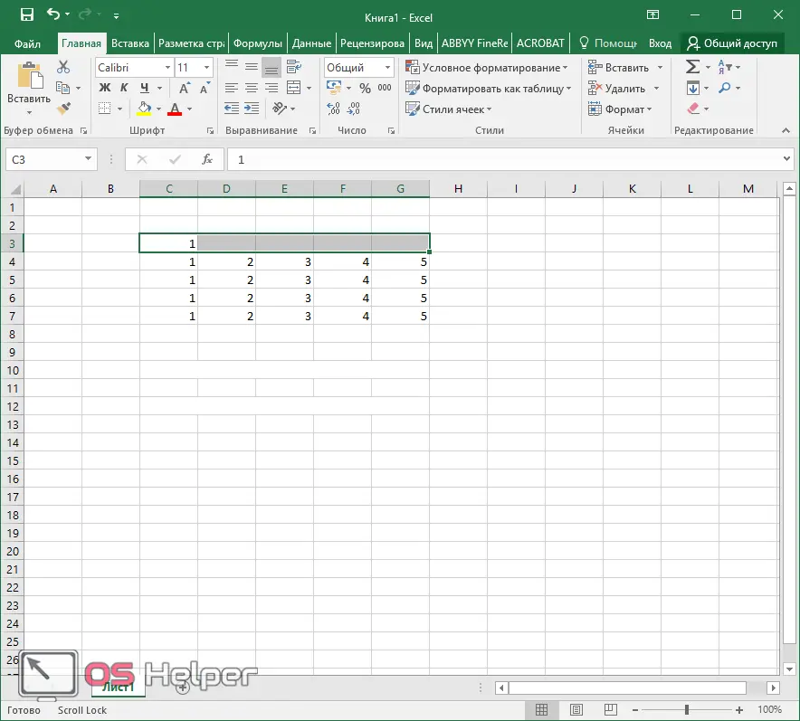
Context menu

You can also do the above using the context menu.

1. We also first select a long string.
2. Do the right mouse click.
3. Select "Format Cells".

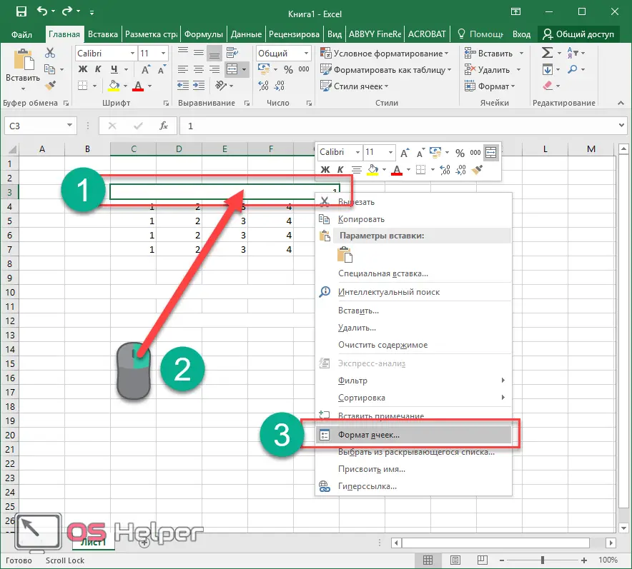
4. In the window that appears, uncheck the box and click on the "OK" button.

5. Thanks to this, everything returns to the way it was originally.

What to do if the button is disabled

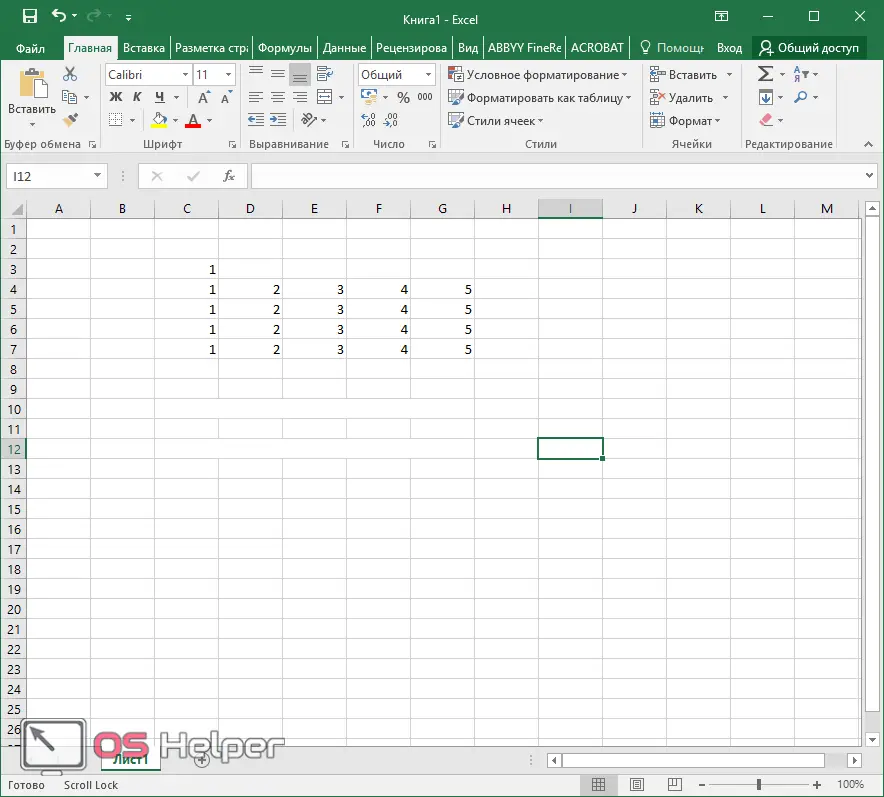
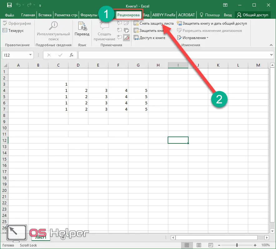
In some cases, it is not possible to edit tables. It has to do with protecting the sheet. It's very easy to remove it.

Go to the "Review" tab and click on the "Unprotect sheet" button.

Conclusion

The methods described in this article for combining rows and columns in Excel are suitable for all modern versions of the application (starting from 2007). If something does not work out for you, you may not have read the instructions carefully. The reason may be that you select the wrong elements. Or don't highlight them at all.

Video instruction

For those who still have any questions, a video is attached below, in which you can hear additional comments.